1.1 Limiting cases

One of the most interesting features of the CGLE is that it interpolates between two well-known limits: a variational system and the nonlinear Schrödinger equation.

1.1.1 Variational formulation

Let us consider the special case where and transform to a rotating frame:

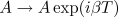
then the CGLE becomes

This equation can then be written in the form

where

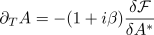
We can now see that

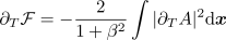
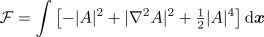
Thus, for finite , the value of the functional assumes the role of a Lyapunov functional (or free energy). Since it is bounded from below, the system then relaxes towards the local minima.

1.1.2 Hamiltonian formulation

In the limit of , (and after some rescaling) the CGLE transforms into the nonlinear Schrödinger equation

which is both Hamiltonian and integrable (it possesses well-known soliton solutions). Indeed, the CGLE can be thought of as a dissipative extension of the conservative nonlinear Schrödinger equation.

One of the aspects of the CGLE that makes it so interesting is the fact that in general, the equation is neither relaxational or Hamiltonian, but can display dynamics characteristic of both types of system. One means of analysing the CGLE is to use these two limits as starting points for the application of perturbation theory.