2.2 Plane waves: simulations

Here we illustrate the theoretical results of the previous page by simulating the CGLE using pseudospectral code with periodic boundary conditions. The MATLAB file that was used to generate these images is available for download from the resources page.

Let us begin by visualising plane waves. If we choose and such that there exists a stable range of wavenumbers then simulate the CGLE with an initial condition of small noise then plane waves are automatically selected.

Space-time plots of , and for . The container size was 200 and the initial condition was noise of order 0.01.

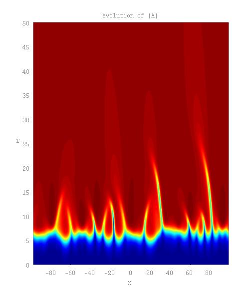
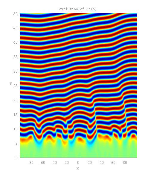
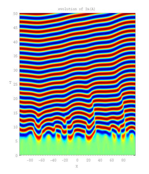
We see that quickly converges to a non-zero constant value. However, as seen in the evolutions of and , the wavenumbers of the newly-selected plane waves do not settle down as quickly. Rather, a much larger time-scale is needed for the wavenumber to be independent of space. Ultimately, the space-time contours will become straight lines.

The Benjamin-Feir instability

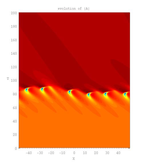
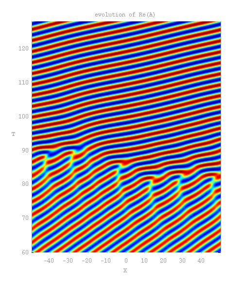
If we now consider the same parameter space but using a linearly unstable plane wave as our initial condition then we can observe the Benjamin-Feir instability:

Space-time plots of and for . The container size was 100 and the initial condition was an unstable plane wave.

Here we see a new plane wave is selected with wavenumber lying inside the band of stability. The process of selecting the new plane wave gives rise to 6 'defects' or phase singularities (points where is zero) where the wavenumber of the plane wave is altered by a discrete amount. This behaviour matches that of the Eckhaus instability for stationary solutions to the RGLE. A range of other behaviours are possible when the Benjamin-Feir-Newell criterion is violated; a selection of these are documented on the next page.